Detecting Frauds with Machine Learning
The importance of a good feature engineering

As you may know, customer acquisition has become increasingly difficult and complex, which makes cost management even more vital for controlling margins and business growth.
One of the biggest issues of operational costs is the FRAUDS. So dealing with them has become essential in companies’ growth strategy.
Big amounts of financial transactions are made every single day, which increases the complexity to identify frauds among them. According to PSafe (https://www.psafe.com/), 3.6 frauds happened in Brazil every minute in 2019.
In this scenario, AI is a powerful way for companies have to detect frauds robustly and flexibly.
So today I’m bringing here one simple way to build a classifier model with python to identify frauds in a big dataset of transactions.
This solution is part of a series of challenges of the Data Science and Machine Learning course from TERA. The expert responsible for the fraud challenge is Patricia Pampanelli, who works as Deep Learning Solutions Architect at NVIDIA.
The solution can be divided in:
- Exploratory Data Analysis
- Correlation
- Feature engineering
- Model training
- Results verification
The dataset used can be found here, and you can check my whole resolution on my Github.
Exploratory Data Analysis (EDA)
First of all, let’s import the libraries
# importing librariesimport pandas as pd
import numpy as np
import matplotlib.pyplot as plt
import seaborn as sns
from numpy import asarray

from datetime import datetime as dt
from datetime import timedelta as td

from sklearn.preprocessing import OrdinalEncoder
from sklearn.model_selection import train_test_split

# Feature importance
from sklearn.inspection import permutation_importance

import warnings
warnings.filterwarnings("ignore")
Now, we have to import the dataset we’re going to work with
# importing the dataset from Google Drive
from google.colab import drive
drive.mount("/content/gdrive")df = pd.read_csv('/content/gdrive/My Drive/Curso TERA/Desafio Classificação - Fraude/fraud_detection_dataset.csv')# verifing the dataset
df.head()

This dataset has 6362620 lines, 11 features and it doesn’t have any missing data.
Distribution os frauds
The target here is the feature called isFraud, which indicates if the transaction was a fraud (1), or not (0). So, our first analysis is to check the distribution between isFraud feature.
# verifying frauds distribution
plt.figure(figsize = (10,6))

ax = sns.countplot(df.isFraud)
ax.set_title('Distribuição de Fraudes', fontsize = 15)
ax.set_xlabel("")
ax.set_ylabel("")
for p in ax.patches:
    ax.annotate('{:.2f}%'.format(100*p.get_height()/len(df.isFraud)), (p.get_x()+ 0.35, p.get_height()+1000))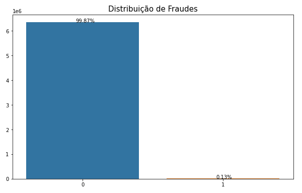
We can notice that the distribution is completely unbalanced, which may require more attention during our modeling.
Frauds over time
The feature step represents the hours of the month during the data acquisition. It ranges from 1 to 743 and it’s not divided into days or months.
# verifying frauds over time
plt.figure(figsize=(15,7))
df.groupby('step')['isFraud'].sum().plot()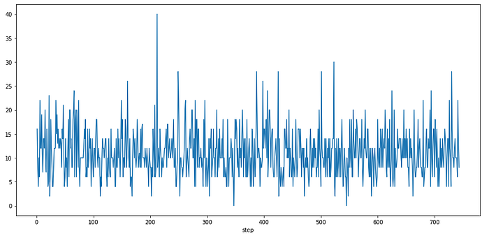
Frauds have an oscillation over the hours, which can indicate that we should work on it later, during feature engineering.
Types of transactions
The feature type represents the kind of transaction that was made. So, let’s check the distribution of types of transactions during frauds.
# types os transactions during frauds
sns.countplot(df[df['isFraud']==1]['type'])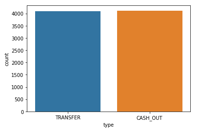
During frauds, only transfer and cash out transactions were made.
Origin and Destiny Names
How often origin names repeat in our dataset?
# quantidade de cada nome da lista de origem
df.nameOrig.value_counts()C1902386530    3
C363736674     3
C545315117     3
C724452879     3
C1784010646    3
              ..
C98968405      1
C720209255     1
C1567523029    1
C644777639     1
C1280323807    1
Name: nameOrig, Length: 6353307, dtype: int64
What about destiny names?
# quantidade de cada nome da lista de destino
df.nameDest.value_counts()C1286084959    113
C985934102     109
C665576141     105
C2083562754    102
C248609774     101
              ...
M1470027725      1
M1330329251      1
M1784358659      1
M2081431099      1
C2080388513      1
Name: nameDest, Length: 2722362, dtype: int64
We can see that there were considerably more transactions for the same destiny names than for origin names. But does it matter? Let’s keep looking for an answer.
How many fraud transactions there were for the same destiny name?
df[df.isFraud==1]['nameDest'].value_counts()C1193568854    2
C104038589     2
C200064275     2
C1497532505    2
C1601170327    2
              ..
C317811789     1
C24324787      1
C1053414206    1
C2013070624    1
C873221189     1
Name: nameDest, Length: 8169, dtype: int64
Oh, it doesn’t seem to be too much…but wait! Only one more question about it.
For those destiny names in frauds, how many transactions did they have?
df_Quant_Trans_Dest = pd.DataFrame({'names_Dest': df.nameDest.value_counts().index.tolist(),
                                    'quantTrans': df.nameDest.value_counts()}).reset_index()name_dest_fraudes = df[df.isFraud==1]['nameDest'].value_counts().index.tolist()df_Quant_Trans_Dest_Frauds = df_Quant_Trans_Dest[df_Quant_Trans_Dest['names_Dest'].isin(name_dest_fraudes)].drop('index', axis=1)df_Quant_Trans_Dest_Frauds.reset_index(inplace=True)df_Quant_Trans_Dest_Frauds.drop('index', axis=1, inplace=True)df_Quant_Trans_Dest_Frauds
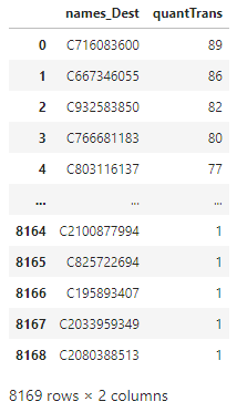
The distribution is:
sns.boxplot(df_Quant_Trans_Dest_Frauds['quantTrans'])
It means that 50% of destiny names of fraud transactions had from 1 to 11 transactions in total. But is it different from those with regular transactions? Let’s check it out.
# dest names with regular transactions (non frauds)
df_Quant_Trans_Dest_NFrauds = df_Quant_Trans_Dest[~df_Quant_Trans_Dest['names_Dest'].isin(name_dest_fraudes)].drop('index', axis=1)df_Quant_Trans_Dest_NFrauds.reset_index(inplace=True)df_Quant_Trans_Dest_NFrauds.drop('index', axis=1, inplace=True)# boxplot of destnames with regular transactions
sns.boxplot(df_Quant_Trans_Dest_NFrauds['quantTrans'])

From this boxplot, we can see that 50% of those destiny names with regular transactions had only 1 transaction in total.
From this names analysis, we can conclude that the number of transactions for destiny names may be a good feature to be considered.
Obs: the same was done for the origin names, but the total transactions of regular and fraud transactions weren’t different. So, the number of transactions didn’t seem to be important in this case.
Correlation
We can easily check the correlation of numeric features with this code.
# ploting the heatmap of correlation
plt.figure(figsize=(10,8))
sns.heatmap(round(df.corr(),4),
            annot=True)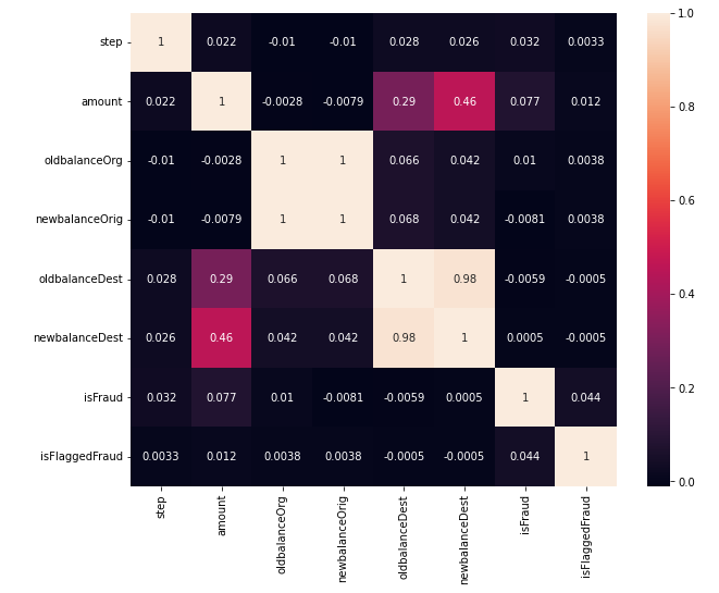
From the correlation, it’s evident that some features are too correlated, as newbalanceDest with oldbalanceDest and amount. So, for our models, we can consider to remove newbalanceDest from the dataset before training the models.
Feature Engineering
Step
As we saw previously, it seems like frauds oscillate over time. But does it have a periodicity? To have it chacked, first, we must convert step data into full dates data (hours, days, month, and year).
# creating a dataframe of dates
# to transform step into hours# we set hours and date of the beginning of our counting
data_inicio = dt(2021, 1, 1, 0, 0, 0)
datas = [data_inicio] # list to keep the dates

# keepdates ina list
for i in range(1, 743):
    data_inicio += td(seconds=3600)
    datas.append(data_inicio)

df_datas = pd.DataFrame({'dates': datas})
df_datas['step'] = df_datas.index+1
df_datas['hour'] = df_datas['dates'].dt.hour# Remove the datetime object column.
df_datas.drop(['dates'], inplace=True, axis=1)df_datas
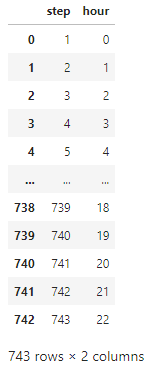
Now, we just have to merge this dates dataframe with our mean dataset.
# merging the mean dataset with dates dataframe

df_com_horas = pd.merge(df_copia, df_datas, on=['step'], how='left')# day hours vs frauds
sns.countplot(df_novas_features[df_novas_features['isFraud']==1]['hour'])
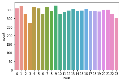
It seems like during day hours frauds don’t oscilate that much. But what about the ratio of frauds?
df_horas_percentual_fraudes = pd.DataFrame({'hour': df_novas_features['hour'].unique(),
                                           'total':df_novas_features.groupby('hour')['isFraud'].count(),
                                           'frauds': df_novas_features.groupby('hour')['isFraud'].sum()})df_horas_percentual_fraudes['frauds_ratio'] = round(df_horas_percentual_fraudes['frauds']/df_horas_percentual_fraudes['total'],2)df_horas_percentual_fraudes.drop('hour', axis=1, inplace=True)df_horas_percentual_fraudes.frauds_ratio.plot()
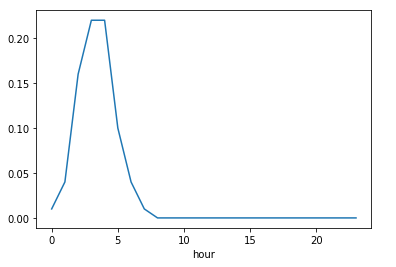
From hours 0 to 8, we have a higher ratio of frauds than the other hours of the day. So, let’s create a feature of 0 and 1, representing these two scenarios (from 0 to 8 and from 9 to 23).
NameDest
As explained above, regarding destiny names, we just have to create another feature representing the number of transactions.
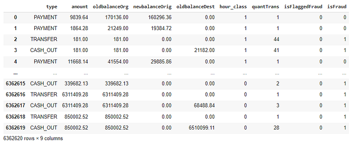
At the end of the feature engineering, we can drop the features: step, nameOrig, nameDest, newbalanceDest, and hour.
So, we’ll have this dataset to use in the modeling
Model Training
Before starting our ML model, we have to preprocess the dataset, so that it runs perfectly during the training.
In this case, the preprocessing is not so difficult, because we had to divide the dataset into training, validation, and test datasets, and encode type features. You can check the functions I used to preprocess the dataset on my GitHub.
One important thing to remember is that every time you preprocess your data, you have to fit in the training dataset and then transform the validation and test datasets. It’s important to avoid data leakage.
So, after importing all important libraries and preprocessing the dataset, we can start training our model.
Once our dataset is big enough, we divided it into training, validation, and test datasets. Also, we weren’t able to run many models, since it would take too long to finish our work. So, we chose Random Forest Classifier, from sklearn, as our model in this case.
We first run the unbalanced dataset, with default parameters as our baseline.
rfc = RandomForestClassifier(random_state=42)rfc.fit(X_train, y_train)
y_pred_train_rfc_baseline = rfc.predict(X_valid)
print(classification_report(y_valid, y_pred_train_rfc_baseline))
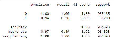
As the first approach, this model seems to be good.
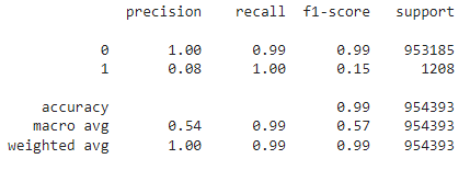
After that, I tried to use the undersampling method to check if we would have a better result, but it didn’t, as it’s shown in the image below.
So now, we just had to optimize the hyperparameters and check the results in the test dataset. In this case, I wanted to use GridSearchCV, but it wasn’t possible due to the size of our dataset. So, I just ran Random Forest two times, with different hyperparameters, and chose one of them.
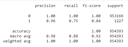
After that, we got the following hyperparameters and used them to predict results in the test dataset. The results are shown below.
rfc = RandomForestClassifier(n_estimators=75,
                             max_depth=20,
                             max_features=0.25,
                             random_state=42)
rfc.fit(X_train, y_train)y_pred_train_rfc_teste = rfc.predict(X_test)
print(classification_report(y_test, y_pred_train_rfc_teste))
# creating confusion matrix for rfc in test dataset
ax = sns.heatmap(confusion_matrix(y_test, y_pred_train_rfc_teste),
                 annot=True,
                 annot_kws={"fontsize":10},
                 fmt = 'd',
                 cmap = 'Blues')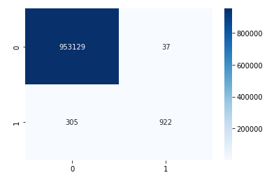
It’s also important to analyse the ROC plot.
y_proba_teste_rfc = rfc.predict_proba(X_test)
y_proba_teste_rfc = y_proba_teste_rfc[:, 1]print('Random Forest Classifier TESTE score:',
      round(rfc.score(X_test, y_test)*100,2))
print('-'*90)roc_auc_rfc = roc_auc_score(y_test, y_proba_teste_rfc)fpr_rfc, tpr_rfc, thresold_rfc = roc_curve(y_test, y_proba_teste_rfc)plt.figure(figsize = (10,10))plt.plot(fpr_rfc, tpr_rfc, color='Red',
        lw=2, label='Random Forest Classifier TESTE\nROC curve (area = %0.2f)' % round(roc_auc_score(y_test, y_proba_teste_rfc)*100,2))plt.plot([0, 1], [0, 1], color='navy', lw=2, linestyle='--')
plt.xlim([0.0, 1.0])
plt.ylim([0.0, 1.05])
plt.xlabel('False Positive Rate')
plt.ylabel('True Positive Rate')
plt.title('Receiver operating characteristic\nFrauds')
plt.legend(loc="lower right")
plt.show()

The area under the curve is 99.81, which is a good result.
Of course, more could be done to have better results for recall, but what I wanted in this project was to show the importance of good feature engineering and also point out some examples of what we can find during data exploration
Conclusion
At the end of this project, I noticed that feature engineering was essential for the good results we got. It’s a good lesson we take from this work: it’s not only about modeling, it’s about understanding what the data tells you before starting throwing them inside ML models.
I really hope this explanation will help you in some way! If you have any questions, feel free to leave a comment, or you can find me on Linkedin.
